Loss Functions
Cross-Entropy
Cross-entropy loss, or log loss, measures the performance of a classification model whose output is a probability value between 0 and 1. Cross-entropy loss increases as the predicted probability diverges from the actual label. So predicting a probability of .012 when the actual observation label is 1 would be bad and result in a high loss value. A perfect model would have a log loss of 0.
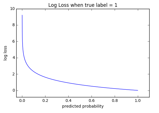
The graph above shows the range of possible loss values given a true observation (isDog = 1). As the predicted probability approaches 1, log loss slowly decreases. As the predicted probability decreases, however, the log loss increases rapidly. Log loss penalizes both types of errors, but especially those predictions that are confident and wrong!
Cross-entropy and log loss are slightly different depending on context, but in machine learning when calculating error rates between 0 and 1 they resolve to the same thing.
Code
Math
In binary classification, where the number of classes \(M\) equals 2, cross-entropy can be calculated as:
If \(M > 2\) (i.e. multiclass classification), we calculate a separate loss for each class label per observation and sum the result.
Note
- M - number of classes (dog, cat, fish)
- log - the natural log
- y - binary indicator (0 or 1) if class label \(c\) is the correct classification for observation \(o\)
- p - predicted probability observation \(o\) is of class \(c\)
Huber
Typically used for regression. It’s less sensitive to outliers than the MSE as it treats error as square only inside an interval.
Code
Further information can be found at Huber Loss in Wikipedia.
Kullback-Leibler
Code
RMSE
Root Mean Square Error
Code
MAE (L1)
Mean Absolute Error, or L1 loss. Excellent overview below [6] and [10].
Code
MSE (L2)
Mean Squared Error, or L2 loss. Excellent overview below [6] and [10].
References
| [1] | https://en.m.wikipedia.org/wiki/Cross_entropy |
| [2] | https://www.kaggle.com/wiki/LogarithmicLoss |
| [3] | https://en.wikipedia.org/wiki/Loss_functions_for_classification |
| [4] | http://www.exegetic.biz/blog/2015/12/making-sense-logarithmic-loss/ |
| [5] | http://neuralnetworksanddeeplearning.com/chap3.html |
| [6] | http://rishy.github.io/ml/2015/07/28/l1-vs-l2-loss/ |
| [7] | https://en.wikipedia.org/wiki/S%C3%B8rensen%E2%80%93Dice_coefficient |
| [8] | https://en.wikipedia.org/wiki/Huber_loss |
| [9] | https://en.wikipedia.org/wiki/Hinge_loss |
| [10] | http://www.chioka.in/differences-between-l1-and-l2-as-loss-function-and-regularization/ |