Classification Algorithms
Classification problems is when our output Y is always in categories like positive vs negative in terms of sentiment analysis, dog vs cat in terms of image classification and disease vs no disease in terms of medical diagnosis.
Bayesian
Overlaps..
Decision Trees
Intuitions
Decision tree works by successively splitting the dataset into small segments until the target variable are the same or until the dataset can no longer be split. It’s a greedy algorithm which make the best decision at the given time without concern for the global optimality [2].
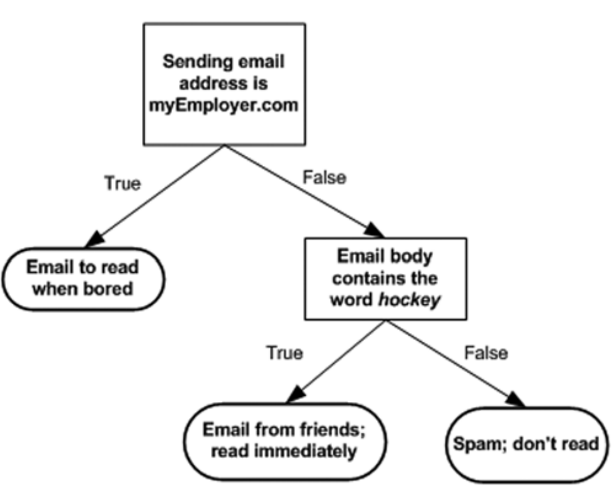
The concept behind decision tree is straightforward. The following flowchart show a simple email classification system based on decision tree. If the address is “myEmployer.com”, it will classify it to “Email to read when bored”. Then if the email contains the word “hockey”, this email will be classified as “Email from friends”. Otherwise, it will be identified as “Spam: don’t read”. Image source [2].
Algorithm Explained
There are various kinds of decision tree algorithms such as ID3 (Iterative Dichotomiser 3), C4.5 and CART (Classification and Regression Trees). The constructions of decision tree are similar [6]:
- Assign all training instances to the root of the tree. Set current node to root node.
- Find the split feature and split value based on the split criterion such as information gain, information gain ratio or gini coefficient.
- Partition all data instances at the node based on the split feature and threshold value.
- Denote each partition as a child node of the current node.
- For each child node:
- If the child node is “pure” (has instances from only one class), tag it as a leaf and return.
- Else, set the child node as the current node and recurse to step 2.
ID3 creates a multiway tree. For each node, it trys to find the categorical feature that will yield the largest information gain for the target variable.
C4.5 is the successor of ID3 and remove the restriction that the feature must be categorical by dynamically define a discrete attribute that partitions the continuous attribute in the discrete set of intervals.
CART is similar to C4.5. But it differs in that it constructs binary tree and support regression problem [3].
The main differences are shown in the following table:
| Dimensions | ID3 | C4.5 | CART |
| Split Criterion | Information gain | Information gain ratio (Normalized information gain) | Gini coefficient for classification problems |
| Types of Features | Categorical feature | Categorical & numerical features | Categorical & numerical features |
| Type of Problem | Classification | Classification | Classification & regression |
| Type of Tree | Mltiway tree | Mltiway tree | Binary tree |
Code Implementation
We used object-oriented patterns to create the code for ID3, C4.5 and CART. We will first introduce the base class for these three algorithms, then we explain the code of CART in details.
First, we create the base class TreeNode class and DecisionTree
class TreeNode:
    def __init__(self, data_idx, depth, child_lst=[]):
        self.data_idx = data_idx
        self.depth = depth
        self.child = child_lst
        self.label = None
        self.split_col = None
        self.child_cate_order = None

    def set_attribute(self, split_col, child_cate_order=None):
        self.split_col = split_col
        self.child_cate_order = child_cate_order

    def set_label(self, label):
        self.label = label
class DecisionTree()
    def fit(self, X, y):
        """
        X: train data, dimensition [num_sample, num_feature]
        y: label, dimension [num_sample, ]
        """
        self.data = X
        self.labels = y
        num_sample, num_feature = X.shape
        self.feature_num = num_feature
        data_idx = list(range(num_sample))
        # Set the root of the tree
        self.root = TreeNode(data_idx=data_idx, depth=0, child_lst=[])
        queue = [self.root]
        while queue:
            node = queue.pop(0)
            # Check if the terminate criterion has been met
            if node.depth>self.max_depth or len(node.data_idx)==1:
                # Set the label for the leaf node
                self.set_label(node)
            else:
                # Split the node
                child_nodes = self.split_node(node)
                if not child_nodes:
                    self.set_label(node)
                else:
                    queue.extend(child_nodes)
The CART algorithm, when constructing the binary tree, will try searching for the feature and threshold that will yield the largest gain or the least impurity. The split criterion is a combination of the child nodes’ impurity. For the child nodes’ impurity, gini coefficient or information gain are adopted in classification. For regression problem, mean-square-error or mean-absolute-error are used. Example codes are showed below. For more details about the formulas, please refer to Mathematical formulation for decision tree in scikit-learn documentation
class CART(DecisionTree):

    def get_split_criterion(self, node, child_node_lst):
        total = len(node.data_idx)
        split_criterion = 0
        for child_node in child_node_lst:
            impurity = self.get_impurity(child_node.data_idx)
            split_criterion += len(child_node.data_idx) / float(total) * impurity
        return split_criterion

    def get_impurity(self, data_ids):
        target_y = self.labels[data_ids]
        total = len(target_y)
        if self.tree_type == "regression":
            res = 0
            mean_y = np.mean(target_y)
            for y in target_y:
                res += (y - mean_y) ** 2 / total
        elif self.tree_type == "classification":
            if self.split_criterion == "gini":
                res = 1
                unique_y = np.unique(target_y)
                for y in unique_y:
                    num = len(np.where(target_y==y)[0])
                    res -= (num/float(total))**2
            elif self.split_criterion == "entropy":
                unique, count = np.unique(target_y, return_counts=True)
                res = 0
                for c in count:
                    p = float(c) / total
                    res -= p * np.log(p)
        return res
K-Nearest Neighbor
Introduction
K-Nearest Neighbor is a supervised learning algorithm both for classification and regression. The principle is to find the predefined number of training samples closest to the new point, and predict the label from these training samples [1].
For example, when a new point comes, the algorithm will follow these steps:
- Calculate the Euclidean distance between the new point and all training data
- Pick the top-K closest training data
- For regression problem, take the average of the labels as the result; for classification problem, take the most common label of these labels as the result.
Code
Below is the Numpy implementation of K-Nearest Neighbor function. Refer to code example for details.
def KNN(training_data, target, k, func):
    """
    training_data: all training data point
    target: new point
    k: user-defined constant, number of closest training data
    func: functions used to get the the target label
    """
    # Step one: calculate the Euclidean distance between the new point and all training data
    neighbors= []
    for index, data in enumerate(training_data):
        # distance between the target data and the current example from the data.
        distance = euclidean_distance(data[:-1], target)
        neighbors.append((distance, index))

    # Step two: pick the top-K closest training data
    sorted_neighbors = sorted(neighbors)
    k_nearest = sorted_neighbors[:k]
    k_nearest_labels = [training_data[i][1] for distance, i in k_nearest]

    # Step three: For regression problem, take the average of the labels as the result;
    #             for classification problem, take the most common label of these labels as the result.
    return k_nearest, func(k_nearest_labels)
Logistic Regression
please refer to logistic regresion
Random Forests
Random Forest Classifier using ID3 Tree: code example
Boosting
Boosting is a powerful approach to increase the predictive power of classification and regression models. However, the algorithm itself can not predict anything. It is built above other (weak) models to boost their accuracy. In this section we will explain it w.r.t. a classification problem.
In order to gain an understanding about this topic, we will go briefly over ensembles and learning with weighted instances.
Excurse:
Ensembles
Boosting belongs to the ensemble family which contains other techniques like bagging (e.i. Random Forest classifier) and Stacking (refer to mlxtend Documentations). The idea of ensembles is to use the wisdom of the crowd:
- a single classifier will not know everything.
- multiple classifiers will know a lot.
One example that uses the wisdom of the crowd is Wikipedia.
The prerequisites for this technique are:
- different classifiers have different knowledge.
- different classifiers make different mistake.
we can fulfill the first prerequisite by using different datasets that are collected form different resources and in different times. In practice, this is most of the time impossible. Normally, we have only one dataset. We can go around this by using cross validation (See Figure below) and use one fold to train a classifier at a time. The second prerequisite means that the classifiers may make different mistakes. Since we trained our classifiers on different datasets or using cross-validation, this condition is already fulfilled.
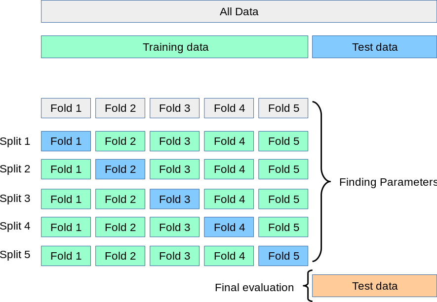
Using cross-validation with ensembles.
Now, we have multiple classifiers, we need a way to combine their results. This actually the reason we have multiple ensemble techniques, they are all based on the same concept. They may differ in some aspects, like whether to use weighted instances or not and how they combine the results for the different classifiers. In general, for classification we use voting and for regression we average the results of the classifiers. There are a lot of variations for voting and average methods, like weighted average. Some will go further and use the classifications or the results from all of the classifier(aka. base-classifiers) as features for an extra classifier (aka. meta classifier) to predict the final result.
learning with weighted instances
For classification algorithms such as KNN, we give the same weight to all instances, which means they are equally important. In practice, instances contribute differently, e.i., sensors that collect information have different quality and some are more reliable than others. We want to encode this in our algorithms by assigning weights to different instances and this can be done as follows:
- changing the classification algorithm (expensive)
- duplicate instances such that an instance with wight n is duplicated n times
Coming back to the actual topic, we can implement boosting, if we train a set of classifiers (not parallel, as the case with Random forest) one after another. The first classifier is a created in a normal way. the latter classifiers have to focus on the misclassified examples by previous ones. How we can achieve this? Well, we can assign weights to instances (learning with weighted instances). If a classifier misclassified an example, we assign higher weight to this example to get more focus from the next classifier(s). Correct examples stay un-touched. It was important to highlight that boosting is an ensemble technique, at the same time, something about boosting might be somehow confusing, in boosting we break the rule of using different datasets, since we want to focus on misclassified examples from previous models, we need to us all data we have to train all models. In this way, a misclassified instance from the first model, will be hopefully classified correctly from the second or the subsequent ones.
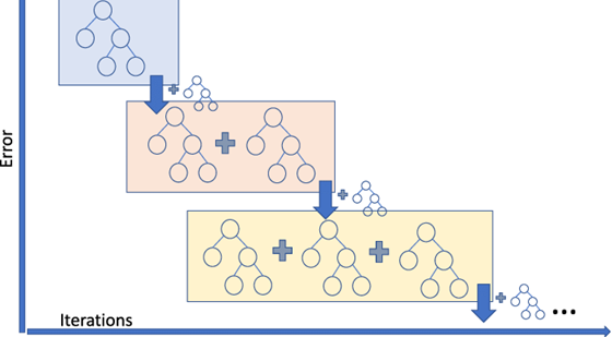
Error decreases with an increasing number of classifiers.
An implementation of the Adaboost (one of the boosting algorithms) from scratch can be found here (python-course.eu) with more details about the algorithm
Support Vector Machine
Support Vector Machine, or SVM, is one of the most popular supervised learning algorithms, and it can be used both for classification as well as regression problems. However, in machine learning, it is primarily used for classification problems. In the SVM algorithm, each data item is plotted as a point in n-dimensional space, where n is the number of features we have at hand, and the value of each feature is the value of a particular coordinate.
The goal of the SVM algorithm is to create the best line, or decision boundary, that can segregate the n-dimensional space into distinct classes, so that we can easily put any new data point in the correct category, in the future. This best decision boundary is called a hyperplane. The best separation is achieved by the hyperplane that has the largest distance to the nearest training-data point of any class. Indeed, there are many hyperplanes that might classify the data. Aas reasonable choice for the best hyperplane is the one that represents the largest separation, or margin, between the two classes.
The SVM algorithm chooses the extreme points that help in creating the hyperplane. These extreme cases are called support vectors, while the SVM classifier is the frontier, or hyperplane, that best segregates the distinct classes.
The diagram below shows two distinct classes, denoted respectively with blue and green points. The maximum-margin hyperplane is the distance between the two parallel hyperplanes: positive hyperplane and negative hyperplane, shown by dashed lines. The maximum-margin hyperplane is chosen in a way that the distance between the two classes is maximised.
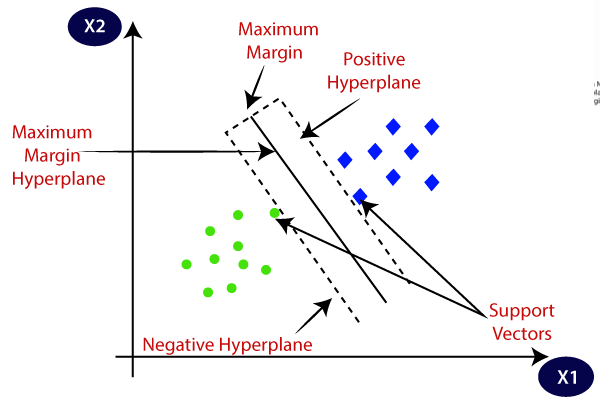
Support Vector Machine: Two different categories classified using a decision boundary, or hyperplane. Source [7]
Support Vector Machine can be of two types:
- Linear SVM: A linear SVM is used for linearly separable data, which is the case of a dataset that can be classified into two distinct classes by using a single straight line.
- Non-linear SVM: A non-linear SVM is used for non-linearly separated data, which means that a dataset cannot be classified by using a straight line.
Linear SVM
Let’s suppose we have a dataset that has two classes, stars and circles. The dataset has two features, x1 and x2. We want a classifier that can classify the pair (x1, x2) of coordinates in either stars or circles. Consider the figure below.
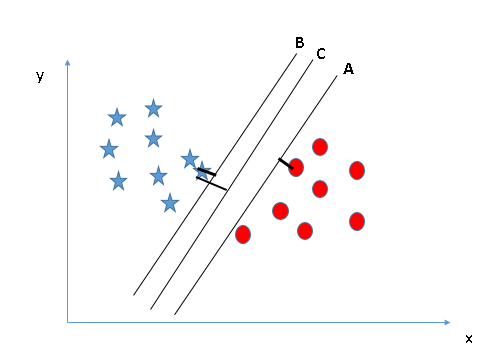
Source [8]
Since it is a 2-dimensional space, we can separate these two classes by using a straight line. The figure shows that we have three hyperplanes, A, B, and C, which are all segregating the classes well. How can we identify the right hyperplane? The SVM algorithm finds the closest point of the lines from both of the classes. These points are called support vectors. The distance between the support vectors and the hyperplane is referred as the margin. The goal of SVM is to maximize this margin. The hyperplane with maximum margin is called the optimal hyperplane. From the figure above, we see that the margin for hyperplane C is higher when compared to both A and B. Therefore, we name C as the (right) hyperplane.
Non-linear SVM
When the data is linearly arranged, we can separate it by using a straight line. However, for non-linear data, we cannot draw a single straight line. Let’s consider the figure below.
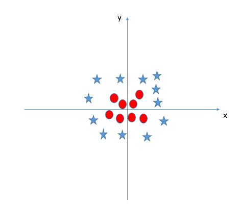
Source [8]
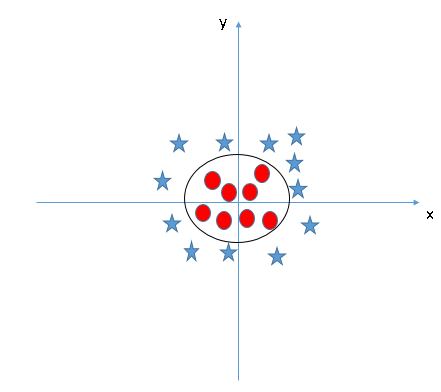
In order to separate the circles from the stars, we need to introduce an additional feature. In case of linear data, we would use the two features x and y. For this non-linear data, we will add a third dimension, z. z is defined as \(z=x^2+y^2\). By adding the third feature, our space will become as below image.

Source [8]
In the above figure, all values for z will always be positive, because z is the squared sum of x and y. Now, the SVM classifier will divide the dataset into two distinct classes by finding a linear hyperplane between these two classes.
Since now we are in a 3-dimensional space, the hyperplane looks like a plane parallel to the x-axis. If we convert it in 2-dimensional space with \(z=1\), then it will become as the figure below.
Source [8]
(Hence, in case of non-linear data, we obtain a circumference of \(radius=1\))
In order to find the hyperplane with the SVM algorithm, we do not need to add this third dimension z manually: the SVM algorithm uses a technique called the “kernel trick”. The SVM kernel is a function which takes a low dimensional input, and it transforms it to a higher dimensional space, i.e., it converts non-linearly separable data to linearly separable data.
References
| [1] | https://scikit-learn.org/stable/modules/neighbors.html#nearest-neighbors-classification |
| [2] | (1, 2) Machine Learning in Action by Peter Harrington |
| [3] | Scikit-learn Documentations: Tree algorithms: ID3, C4.5, C5.0 and CART |
| [4] | Scikit-learn Documentations: Ensemble Method |
| [5] | Medium-article: what is Gradient Boosting |
| [6] | Decision Trees |
| [7] | Support Vector Machine |
| [8] | (1, 2, 3, 4) Support Vector Machine |